Lecture 3

Author

Lifeng Ren

Published

August 16, 2023

Course Updates

Lecture 1’s link is now available on GitHub
Any Questions? Comments? Suggestions?

Recap from Yesterday

Control structures
- Conditional statements (if, else, ifelse)
- Loops (for, while, repeat, break, next)
Functions:
- Introduction to built-in functions
- Writing custom functions
- The apply family of functions (lapply, sapply, tapply, etc.)
Library and Packages
Data Manipulation
- base
- tidyverse
- data.table

Introduction

In this lecture, we will delve into the following topics:

More in Data Cleaning and Wrangling:
- Revisit the Combining Data sets from yesterday
  - merge: base
  - join: dplyr
  - Compare with 1:m, m:1, 1:1 in STATA
- Data Reshaping
  - data.table
- Data Standardization
  - Dates:
  - Text: stringr
- Unique Identifier
Basic Data Analysis and Data Visualization in R
- Preliminary Data Checks
- Simple Regression
- Results and Visualization
A Comprehensive Project in Class
- A review for the last 2.5 days
- Do this in the rmd file I provide you.
- Your output should be a html report

For Tomorrow

Intermediate Econometrics in R Review
- Mathematical Statistics in R
  - Distributions
  - Simulations
- Intermediate Applied Econometrics
  - Testing
  - …

Data Manipulation Again

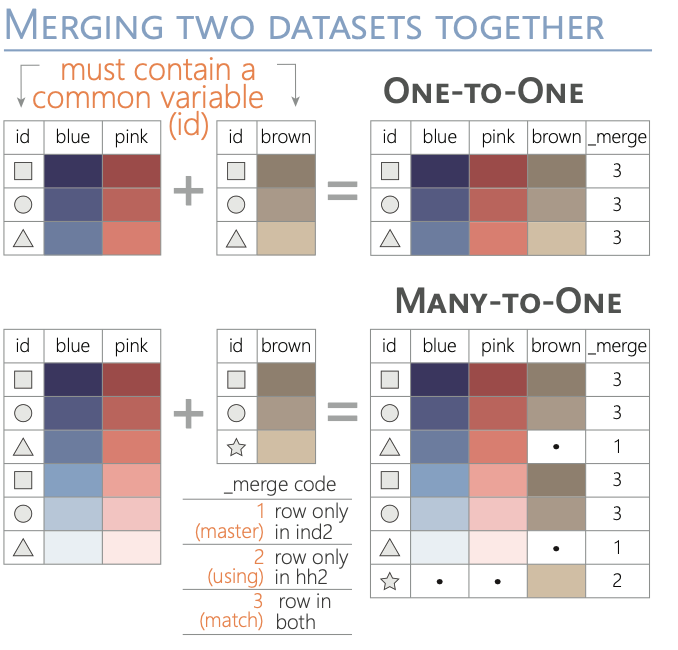
Merge: Comparison with STATA

In STATA, when merging datasets, you specify the type of merge using:

1:1: One-to-one join: Each observation in the dataset has a unique identifier, and each identifier in one dataset matches to one and only one identifier in the other dataset.
1:m: One-to-many join: You start with the “many” dataset. For each unique identifier in the “many” dataset, there’s a corresponding single observation in the “one” dataset. When you perform the merge, each of the multiple observations in the “many” dataset with the same identifier gets matched to a single observation in the “one” dataset.
m:1: Many-to-one join: You start with the “one” dataset. For each unique identifier in the “one” dataset, there are multiple corresponding observations in the “many” dataset. When you perform the merge, the single observation in the “one” dataset gets matched to each of the multiple observations in the “many” dataset with the same identifier.

Let’s use examples to understand the link and difference between merging datasets in R and STATA. We will see two cases: 1) all keys can be matched and 2) some keys cannot be matched:

Demo with R and save the temporary data into a .dta file using the haven library.
Use STATA commands and see if the output matches our expectations.

Every `Key` Exist in Both Data Set

All three should be the same.

R Demo using `base`

Since we need to save datasets, we need to define the working directory and libraries we are going to use as usual.

# setwd("~/Library/CloudStorage/Box-Box/Teaching/R_2023/local/lec3")

library(haven)

One-to-One (1:1) Merge:

df1 <- data.frame(ID = c(1, 2, 3), Name = c("Alice", "Bob", "Charlie"))
df2 <- data.frame(ID = c(1, 2, 3), Age = c(25, 30, 28))

write_dta(df1, "df1.dta")
write_dta(df2, "df2.dta")

merged_df <- merge(df1, df2, by = "ID")
write_dta(merged_df, "one_to_one_merge.dta")

Many-to-One (m:1) Merge:

many_df <- data.frame(ID = c(1, 1, 2, 3), Score = c(85, 90, 88, 92))
one_df <- data.frame(ID = c(1, 2, 3), Name = c("Alice", "Bob", "Charlie"))

write_dta(many_df, "many_df.dta")
write_dta(one_df, "one_df.dta")

merged_df <- merge(many_df, one_df, by = "ID")
write_dta(merged_df, "many_to_one_merge_R.dta")

One-to-Many (1:m) Merge:

(Using the same example datasets as for the m:1 merge)

merged_df <- merge(one_df, many_df, by = "ID")
write_dta(merged_df, "one_to_many_merge_R.dta")

STATA Demo

We should expect the perfect match.

R Demo with dplyr: left_join and right_join

For this case, the results should be the same. Because both many_df and one_df are having information for all IDs. Let us double-check if we are using left_join, right_join in R.

First, we’ll create two data frames: teachers (the “one” dataset) and classes (the “many” dataset). Then, we’ll perform both m:1 and 1:m merges using both left and right joins, and show the results.

Here’s the R code:

# Load the required library
library(dplyr)

# Create the 'teachers' dataframe (the "one" dataset)
teachers <- data.frame(
  TeacherID = c(1, 2),
  TeacherName = c("Mr. Smith", "Mrs. Jones")
)

# Create the 'classes' dataframe (the "many" dataset)
classes <- data.frame(
  ClassID = c("A", "B", "C"),
  ClassName = c("Math", "Science", "English"),
  TeacherID = c(1, 1, 2)
)

# m:1 Merge using left join (starting with 'classes' as the base)
m1_merge_left <- left_join(classes, teachers, by = "TeacherID")

# 1:m Merge using left join (starting with 'teachers' as the base)
# This produces the same result as the m:1 merge but potentially with reordered columns
one_m_merge_left <- left_join(teachers, classes, by = "TeacherID")

# m:1 Merge using right join (starting with 'classes' as the base)
m1_merge_right <- right_join(classes, teachers, by = "TeacherID")

# 1:m Merge using right join (starting with 'teachers' as the base)
one_m_merge_right <- right_join(teachers, classes, by = "TeacherID")

# Print results
list(
  m1_merge_left = m1_merge_left,
  one_m_merge_left = one_m_merge_left,
  m1_merge_right = m1_merge_right,
  one_m_merge_right = one_m_merge_right
)

$m1_merge_left
  ClassID ClassName TeacherID TeacherName
1       A      Math         1   Mr. Smith
2       B   Science         1   Mr. Smith
3       C   English         2  Mrs. Jones

$one_m_merge_left
  TeacherID TeacherName ClassID ClassName
1         1   Mr. Smith       A      Math
2         1   Mr. Smith       B   Science
3         2  Mrs. Jones       C   English

$m1_merge_right
  ClassID ClassName TeacherID TeacherName
1       A      Math         1   Mr. Smith
2       B   Science         1   Mr. Smith
3       C   English         2  Mrs. Jones

$one_m_merge_right
  TeacherID TeacherName ClassID ClassName
1         1   Mr. Smith       A      Math
2         1   Mr. Smith       B   Science
3         2  Mrs. Jones       C   English

Just like before, everything matched!

Some `keys` cannot be matched

Now, let us see the behavior of left_join when there’s no match for a record in either the left or the right table, and we want this being demonstrated using both dplyr and base R.

Let’s slightly modify our datasets to have unmatched records:

In the teachers dataframe, let’s add a teacher with TeacherID = 3 named “Mr. Doe” who doesn’t have any associated class.
In the classes dataframe, let’s add a class with ClassID = "D" named “History” with TeacherID = 4, but there’s no teacher with TeacherID = 4 in the teachers dataframe.

Now, let’s perform the left joins using both dplyr and base R:

Using dplyr:

Perform left_join using classes as the base.
Perform left_join using teachers as the base.

Using base R:

Use merge with all.x = TRUE using classes as the base.
Use merge with all.x = TRUE using teachers as the base.

# Modify the datasets
teachers_modified <- rbind(teachers, data.frame(TeacherID = 3, TeacherName = "Mr. Doe"))
classes_modified <- rbind(classes, data.frame(ClassID = "D", ClassName = "History", TeacherID = 4))

# Using dplyr:
dplyr_classes_base <- left_join(classes_modified, teachers_modified, by = "TeacherID")
dplyr_teachers_base <- left_join(teachers_modified, classes_modified, by = "TeacherID")

# Using base R:
base_classes_base <- merge(classes_modified, teachers_modified, by = "TeacherID", all.x = TRUE)
base_teachers_base <- merge(teachers_modified, classes_modified, by = "TeacherID", all.x = TRUE)

list(
  dplyr_classes_base = dplyr_classes_base,
  dplyr_teachers_base = dplyr_teachers_base,
  base_classes_base = base_classes_base,
  base_teachers_base = base_teachers_base
)

$dplyr_classes_base
  ClassID ClassName TeacherID TeacherName
1       A      Math         1   Mr. Smith
2       B   Science         1   Mr. Smith
3       C   English         2  Mrs. Jones
4       D   History         4        <NA>

$dplyr_teachers_base
  TeacherID TeacherName ClassID ClassName
1         1   Mr. Smith       A      Math
2         1   Mr. Smith       B   Science
3         2  Mrs. Jones       C   English
4         3     Mr. Doe    <NA>      <NA>

$base_classes_base
  TeacherID ClassID ClassName TeacherName
1         1       A      Math   Mr. Smith
2         1       B   Science   Mr. Smith
3         2       C   English  Mrs. Jones
4         4       D   History        <NA>

$base_teachers_base
  TeacherID TeacherName ClassID ClassName
1         1   Mr. Smith       A      Math
2         1   Mr. Smith       B   Science
3         2  Mrs. Jones       C   English
4         3     Mr. Doe    <NA>      <NA>

NOTES:

In both the dplyr and base R results, we can observe that where there’s no match for a record in the left table, NA values are filled in for columns from the right table. Which should be similar to the m:1 results from STATA’s picture below. (NOT EXACT THE SAME BUT SAME IDEA)

Reshaping

`Base` R Methods:

reshape Function:

Base R provides the reshape function, which can convert data from wide to long format and vice versa.

Wide to Long:

  # Sample data
  data <- data.frame(
    ID = 1:3,
    Time1 = c(5, 6, 7),
    Time2 = c(8, 9, 10)
  )

  print(data)

  ID Time1 Time2
1  1     5     8
2  2     6     9
3  3     7    10

  # Reshaping to long format
  long_data <- reshape(data, direction = "long", varying = list(c("Time1", "Time2")), 
                     v.names = "Value", idvar = "ID", timevar = "Time")
  print(long_data)

    ID Time Value
1.1  1    1     5
2.1  2    1     6
3.1  3    1     7
1.2  1    2     8
2.2  2    2     9
3.2  3    2    10

Long to Wide:

    # Reshaping to wide format
    wide_data <- reshape(long_data, direction = "wide", v.names = "Value", 
                     idvar = "ID", timevar = "Time")
    print(wide_data)

    ID Value.1 Value.2
1.1  1       5       8
2.1  2       6       9
3.1  3       7      10

Using `data.table`:

The data.table library offers an efficient and flexible approach to data reshaping, especially for large datasets.

Melting (Wide to Long):

library(data.table)

# Convert data frame to data table
DT <- as.data.table(data)

# Melt to long format
melted_data <- melt(DT, id.vars = "ID", measure.vars = c("Time1", "Time2"), 
                    variable.name = "Time", value.name = "Value")
print(melted_data)

      ID   Time Value
   <int> <fctr> <num>
1:     1  Time1     5
2:     2  Time1     6
3:     3  Time1     7
4:     1  Time2     8
5:     2  Time2     9
6:     3  Time2    10

Casting (Long to Wide):

# Cast to wide format
casted_data <- dcast(melted_data, ID ~ Time, value.var = "Value")
print(casted_data)

Key: <ID>
      ID Time1 Time2
   <int> <num> <num>
1:     1     5     8
2:     2     6     9
3:     3     7    10

Remember, the choice between base R and data.table methods often depends on your specific needs. data.table is especially powerful for large datasets due to its efficiency, while base R can be simpler for basic reshaping tasks or for those who are more familiar with its syntax.

Dates

Date data can be tricky due to various formats and conventions across the world.
Proper handling is essential for chronological analysis, time series forecasting, and event tracking.
Sys.Date(): Returns the current date.
as.Date(): Converts a character string into a Date object.
format(): Formats a Date object into a desired character representation.

Examples

# Current date
current_date <- Sys.Date()
print(current_date)

[1] "2025-09-17"

# Convert a string to a date
date_str <- "2023-08-16"
converted_date <- as.Date(date_str)
print(converted_date)

[1] "2023-08-16"

# Format a date
formatted_date <- format(current_date, format="%B %d, %Y")
print(formatted_date)

[1] "September 17, 2025"

# Define starting and ending dates
start_date <- as.Date("2023-01-01")
end_date <- as.Date("2023-01-10")

# Create a sequence of dates
date_seq <- seq(start_date, end_date, by="days")

# Convert the sequence to a data frame
date_df <- data.frame(Date = date_seq)

# Print the data frame
print(date_df)

         Date
1  2023-01-01
2  2023-01-02
3  2023-01-03
4  2023-01-04
5  2023-01-05
6  2023-01-06
7  2023-01-07
8  2023-01-08
9  2023-01-09
10 2023-01-10

Strings

Text data often contains noise in the form of special characters, inconsistencies in formatting, and more. Properly cleaning and manipulating such data is crucial.

The stringr package in R offers a host of functions that can aid in this.
gsub in base R can do a lot similar functions, I will leave that to you for the future study. Some examples have been provided in the Appendix Section.

Removing Special Characters

Special characters can be noise in some analyses.
Removing them can simplify text and aid in other text processing tasks.
str_replace_all(): Replaces all instances of a pattern in a string.

Examples

library(stringr)

text <- "Hello, world! This is a test. #Test123"
cleaned_text <- str_replace_all(text, "[^[:alnum:][:space:]]", "")
print(cleaned_text)

[1] "Hello world This is a test Test123"

String Matching

Useful to detect if a string contains certain patterns or characters.
str_detect(): Detects the presence or absence of a pattern in a string.
str_which(): Returns the indices of strings that match a pattern.
str_match(): Extract matched groups from a string based on a pattern.

Examples

# Detect if a string contains "world"
text <- c("Hello world", "Hello R", "R is a world of statistics")
print(str_detect(text, "world"))

[1]  TRUE FALSE  TRUE

# Get indices of strings that contain "R"
print(str_which(text, "R"))

[1] 2 3

# Extract matched groups
pattern <- "(\\d{4})-(\\d{2})-(\\d{2})"
date_str <- "Today's date is 2023-08-16."
print(str_match(date_str, pattern))

     [,1]         [,2]   [,3] [,4]
[1,] "2023-08-16" "2023" "08" "16"

Case Conversion

To ensure uniformity in text data.
str_to_upper(): Converts strings to upper case.
str_to_lower(): Converts strings to lower case.
str_to_title(): Converts strings to title case.

Examples

text <- "Hello, World!"

print(str_to_upper(text))

[1] "HELLO, WORLD!"

print(str_to_lower(text))

[1] "hello, world!"

print(str_to_title(text))

[1] "Hello, World!"

Splitting Strings

To break a string into parts based on a delimiter.
str_split(): Splits a string into parts.

Examples

text <- "apple,banana,grape"
print(str_split(text, ","))

[[1]]
[1] "apple"  "banana" "grape"

Other `stringr` functions in R with examples

str_length(): Computes the length of a string.
str_c(): Concatenates strings.
str_sub(): Extracts or replaces substrings.

library(stringr)

# String length
print(str_length("Hello, world!"))

[1] 13

# Concatenate
print(str_c("Hello", "world", sep=", "))

[1] "Hello, world"

# Substring
print(str_sub("Hello, world!", 1, 5))

[1] "Hello"

Unique Identifiers in R

A unique identifier (UID) is an identifier that ensures distinctness among all other items.
UIDs are crucial for indexing, referencing, and joining datasets without confusion.

Functions to Identify Unique and Duplicate Values

unique(): Returns a vector of unique values.

vec <- c(1, 2, 2, 3, 4, 4, 4, 5)
unique_vals <- unique(vec)
print(unique_vals)

[1] 1 2 3 4 5

duplicated(): Returns a logical vector indicating whether an element is a duplicate.

vec <- c(1, 2, 2, 3, 4, 4, 4, 5)
dupes <- duplicated(vec)
print(dupes)

[1] FALSE FALSE  TRUE FALSE FALSE  TRUE  TRUE FALSE

distinct() from the dplyr package: Used to remove duplicate rows from a data frame or tibble.

library(dplyr)
df <- data.frame(name = c("Alice", "Bob", "Alice", "Charlie"), age = c(25, 30, 25, 35))
distinct_df <- distinct(df)
print(distinct_df)

     name age
1   Alice  25
2     Bob  30
3 Charlie  35

Generating Unique Identifiers

seq_along(): Generate a sequence along an object’s length.

vec <- c("apple", "banana", "cherry")
uids <- seq_along(vec)
print(uids)

[1] 1 2 3

make.unique(): Generates unique strings by appending numbers.

vec <- c("apple", "apple", "banana")
unique_vec <- make.unique(vec)
print(unique_vec)

[1] "apple"   "apple.1" "banana"

Checking for Unique Identifiers with `isid()`

The isid() function checks if a given set of variables uniquely identifies the observations in a dataset. Just like the one we are using in STATA.

You need to install eeptools package for this.

library(eeptools)
df <- data.frame(id = c(1, 2, 3, 1), value = c(10, 20, 30, 40))
# Check if 'id' uniquely identifies the data
isid(df, "id", verbose = TRUE)

Are variables a unique ID?
[1] FALSE
Variables define this many unique rows:
[1] 3
There are this many total rows in the data:
[1] 4

In this example, the isid() function would return FALSE because the ‘id’ variable does not uniquely identify each row in the dataset.

Considerations

When working with large datasets or datasets that will be merged, it’s essential to ensure that the data’s unique identifiers remain consistent.
Always check for the uniqueness of identifiers, especially before operations like joining or merging datasets, to prevent unintended duplications or omissions.

Basic Data Analysis and Data Visulizations in R

Preliminary Checks

Before diving into any data analysis, it’s essential to understand and clean your data. This involves checking for outliers, handling missing values, and visualizing data distributions.

For our demonstration, we’ll use the mtcars dataset.
```
  data(mtcars)
```

Checking for Outliers

Outliers can significantly affect regression results. A simple way to check for outliers is by using boxplots.

boxplot(mtcars$mpg, main="Boxplot of MPG", ylab="Miles Per Gallon")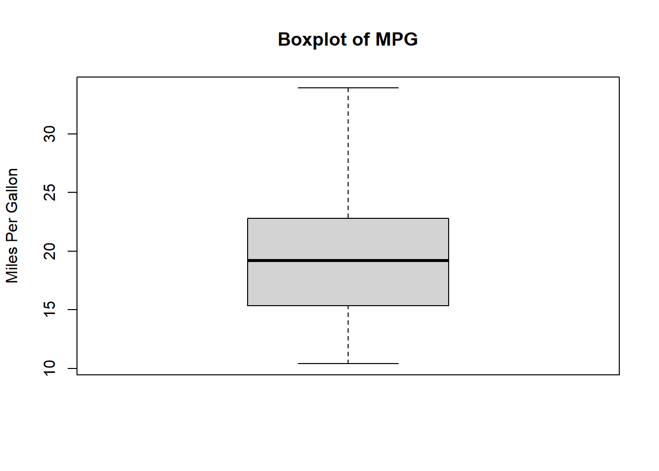

Points outside the “whiskers” of the boxplot could be potential outliers.

Handling Missing Values

Data often comes with missing values, and it’s crucial to handle them appropriately.

Identifying Missing Values

Use is.na() to identify missing values:

    missing_vals <- is.na(mtcars$mpg)
    sum(missing_vals)

[1] 0

Handling Strategies
- Remove rows with missing values: na.omit()
- Impute missing values using mean, median, or a specific strategy.

Data Visualization

Visualizing your data can help in understanding distributions, relationships, and potential issues.

Histogram: Understand the distribution of a variable.

    hist(mtcars$mpg, main="Histogram of MPG", xlab="Miles Per Gallon", col="lightblue")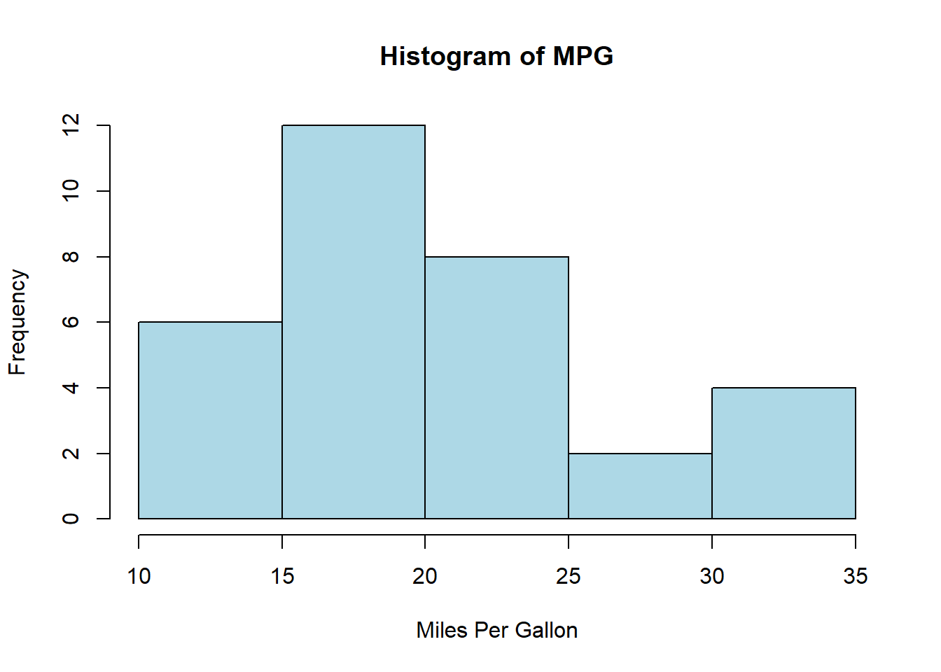

Correlation Plot: Understand relationships between variables.

pairs(mtcars[, 1:4], main="Scatterplot Matrix")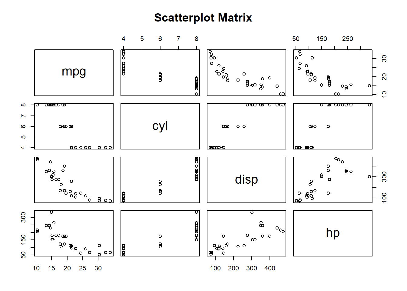

Density Plot: Another way to check the distribution.

  ggplot(mtcars, aes(x=mpg)) + 
    geom_density(fill="blue", alpha=0.5) +
    labs(title="Density Plot of MPG", x="Miles Per Gallon")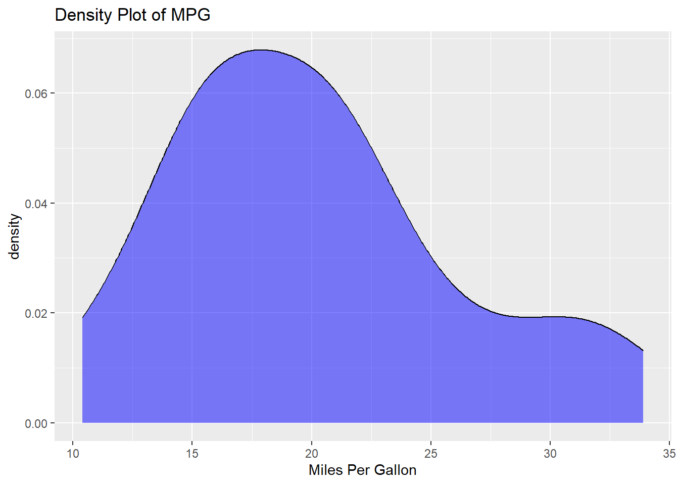

By conducting these preliminary checks, you ensure that your data is ready for deeper analysis, and any insights or results derived are more likely to be reliable.

Data Analysis and Data Visulization (`mtcars` example)

Make sure you’ve installed the packages: tidyverse, lmtest
Done the first-round preliminary data check.

Loading the Libraries

library(tidyverse)
library(lmtest)

Running a Simple Regression in R

A regression allows us to understand relationships between variables. The simplest form is the linear regression, represented as:

\[ Y = \beta_0 + \beta_1 X + \epsilon \]

Where: - $Y$ is the dependent variable. - $X$ is the independent variable. - $\beta_0$ is the intercept. - $\beta_1$ is the slope. - $\epsilon$ is the error term.

model <- lm(mpg ~ wt, data = mtcars)
summary(model)


Call:
lm(formula = mpg ~ wt, data = mtcars)

Residuals:
    Min      1Q  Median      3Q     Max 
-4.5432 -2.3647 -0.1252  1.4096  6.8727 

Coefficients:
            Estimate Std. Error t value Pr(>|t|)    
(Intercept)  37.2851     1.8776  19.858  < 2e-16 ***
wt           -5.3445     0.5591  -9.559 1.29e-10 ***
---
Signif. codes:  0 '***' 0.001 '**' 0.01 '*' 0.05 '.' 0.1 ' ' 1

Residual standard error: 3.046 on 30 degrees of freedom
Multiple R-squared:  0.7528,    Adjusted R-squared:  0.7446 
F-statistic: 91.38 on 1 and 30 DF,  p-value: 1.294e-10

The summary() function provides a detailed summary of the regression results. Here, we are trying to predict mpg (miles per gallon) using the weight (wt) of the car, using the mtcars dataset.

Accessing Regression Results

We can save the summary of the model first:

model_summary <- summary(model)

And we can see that it is a list! This is something we’ve already learned.

From this summary object, you can extract:

coefficients: A matrix where each row represents a predictor (including the intercept) and columns provide details like estimate, standard error, t-value, and p-value.
sigma: The residual standard error.
r.squared: The R-squared value.
adj.r.squared: The adjusted R-squared value.
fstatistic: The F-statistic value and its degrees of freedom.

Access the Coefficients

# Access using summary list
coeff_matrix <- model_summary$coefficients
print(coeff_matrix)

             Estimate Std. Error   t value     Pr(>|t|)
(Intercept) 37.285126   1.877627 19.857575 8.241799e-19
wt          -5.344472   0.559101 -9.559044 1.293959e-10

# Directly access using `coefficients` functions for regression objects
betas <- coefficients(model) # this will give you only the betas
print(betas)

(Intercept)          wt 
  37.285126   -5.344472

Access the Standard Errors

The standard errors of the coefficients can be extracted from the model’s summary object.

standard_errors <- coeff_matrix[, "Std. Error"]
print(standard_errors)

(Intercept)          wt 
   1.877627    0.559101

Access the t-statistics

t_values <- summary(model)$coefficients[, "t value"]
print(t_values)

(Intercept)          wt 
  19.857575   -9.559044

Access the p-values

p_values <- summary(model)$coefficients[, "Pr(>|t|)"]
print(p_values)

 (Intercept)           wt 
8.241799e-19 1.293959e-10

4. Show Basic Regression Figures

Scatter Plot with Regression Line

Visualizing the relationship between the independent and dependent variables can be very insightful.

ggplot(mtcars, aes(x=wt, y=mpg)) +
  geom_point() +
  geom_smooth(method="lm", col="red") +
  labs(title="Relationship between Car Weight and MPG", x="Weight", y="Miles Per Gallon")

`geom_smooth()` using formula = 'y ~ x'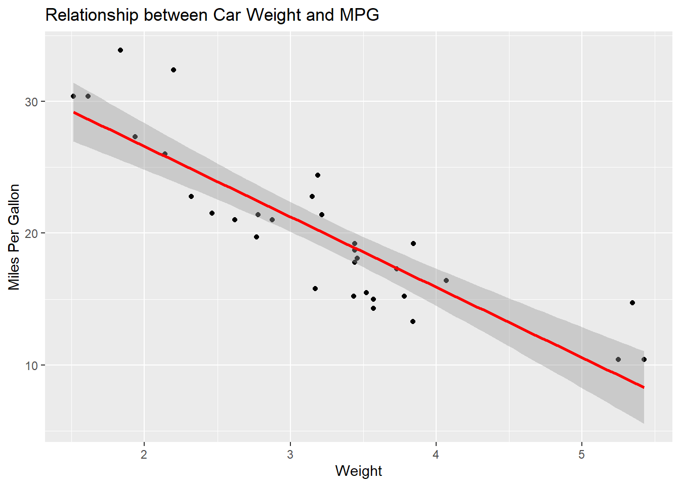

Residuals vs. Fitted Values

Checking the residuals can help diagnose potential issues with the model.

residuals <- resid(model)
fitted_values <- fitted(model)

ggplot() +
  geom_point(aes(x=fitted_values, y=residuals)) +
  labs(title="Residuals vs. Fitted Values", x="Fitted Values", y="Residuals")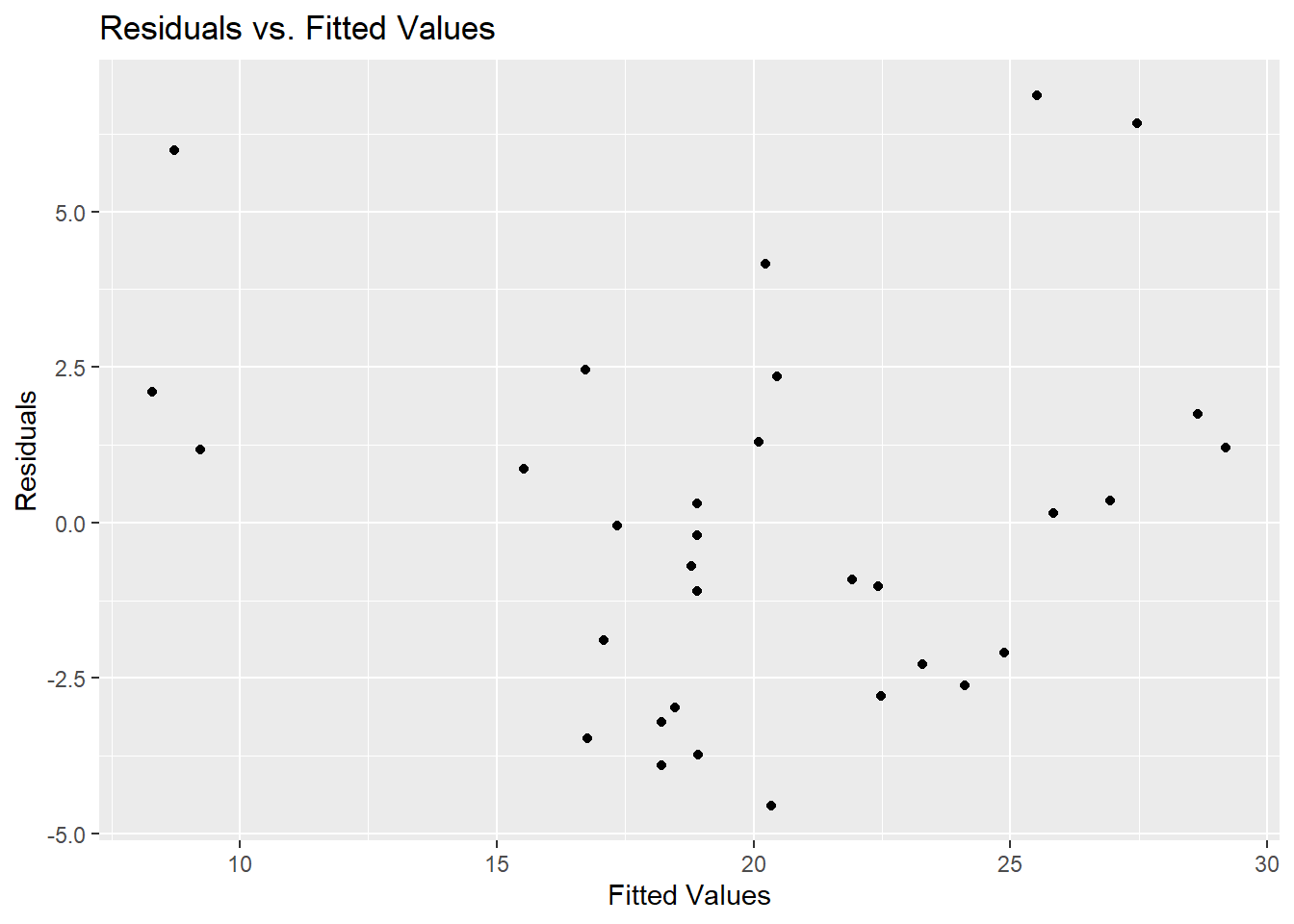

Comprehensive Reivew Project

Introduction

This comprehensive project is designed to review the concepts you’ve learned throughout the course. You’ll apply techniques from data cleaning to advanced data analysis. We’ll work with both built-in datasets and an external dataset.

Datasets

Built-in Dataset: mtcars
External Dataset: “client_data.csv”

Workflows

Create a workflow for this project in the following steps:

Under lec3 folder, create a sub folder lec3_proj
Under lec3_proj folder, create two sub folders: code and data
Under data folder, create three sub folders: raw, temp, and cleaned

Your directories should look like this:

lec3–>
- lec3_proj–>
  - code–>
    - lec3_proj.Rmd
  - data–>
    - raw
    - temp
    - cleaned

Tasks

Preparation

Download the lec3_proj.Rmd from GitHub into your code folder
It is already setup for you with the questions.
Code in the code chunk.
Set up your working directory to the folder ~/lec3/lec3_proj/code/

Data Exploration and Cleaning:
- Generate an external dataset “client_data.csv” with the following code

set.seed(123)

# Number of clients
n_clients <- 200

# 1. Generate 'name' column
client_data <- data.frame(name = paste0("Client_", seq(1, n_clients)))

# 2. Generate 'car_bought' column. Initially, just a random sample
client_data$car_bought <- sample(rownames(mtcars), n_clients, replace = TRUE)

# 3. Generate 'date_purchased' column
client_data$date_purchased <- sample(seq(as.Date('2015/01/01'), as.Date('2022/01/01'), by="day"), n_clients, replace=TRUE)

# 4. Generate 'income' column
client_data$income <- runif(n_clients, min=30000, max=150000)

# 5. Ensure richer clients are more likely to buy cars with more horsepower
# Sort mtcars by horsepower
sorted_cars <- rownames(mtcars[order(mtcars$hp), ])

# Divide clients into groups and assign cars based on sorted horsepower
split_rows <- ceiling(n_clients / length(sorted_cars))
client_data <- client_data[order(-client_data$income), ] # sort by income
client_data$car_bought <- rep(sorted_cars, times = split_rows)[1:n_clients]

# Show the transformed client_data
head(client_data)

# Write the data to a CSV
write.csv(client_data, "../data/raw/client_data.csv", row.names = FALSE)

Load the built-in dataset mtcars. - Create a column named ID, which is the same as the rownames.
Identify missing values using sum, and is.na() function.
Visualize and treat any outliers in the mpg column of the mtcars dataset. - Hint: using boxplot() function, and use ?boxplot() to learn the syntax.

Combining Datasets:
- Merge the datasets using car_ID, and car_bought.
- Use both merge from base and join from dplyr to combine. Discuss the differences.
- Note: the merged dataset should be named as:
- merged_data_base
- merged_data_dplyr
Data Reshaping:
- Use data.table to reshape the merged data set.
- Save the reshaped data set into the temp folder.
- Create a summary table calculating the mean mpg for each unique value in Car_ID.
Data Standardization:
- Standardize any date columns in client_data.csv.
- Purchased Date: as.Date()
- Client’s name: get rid of Client_ using str_replace()
Unique Identifier Check:
- Check if the name is a unique identifier using:
- isid()
- length(unique(DATA$UID))==nrow(DATA)

5.5. Save and Use Cleaned Data to Proceed - Save the “merged_data_base” into the cleaned folder, named as: merged_data_base_cleaned.csv

Regression Analysis:
1. Conducting the Regression:
  - Using the merged dataset, run a regression predicting mpg from another continuous variable.
    - mpg ~ wt
  - Visualize the relationship between the chosen predictor and mpg using a scatter plot.
    - plot(merged_data_base$wt, merged_data_base$mpg, ...)
    - abline()
2. Matrix Operations with Coefficients:
  - Extract the coefficients from the regression model and store them in a matrix.
    - new matrix: matrix()
    - extract coefficients: coefficients(model)
  - Create a 2x2 identity matrix.
    - Use this: identity_matrix <- diag(2)
  - Use matrix multiplication (using %*%) to multiply the identity matrix by the coefficients matrix. The result will be the coefficients themselves.
3. Loops for Analysis (HARD: Don’t Do it for Now):
  - Write a for loop that iterates over the column names of the merged dataset (excluding mpg). In each iteration, run a regression using mpg as the dependent variable and the current column as the independent variable. Store each coefficient in a vector.
  - After the loop, visualize the coefficients using a bar plot to see the impact of each variable on mpg.
4. Interpretation:
  - Discuss the results. Which variables have the most substantial impact on mpg? Are the results consistent with expectations?
Control Structures and Custom Functions:

Use a for loop to calculate the mean of each numeric column in the merged dataset. (HARD: Don’t Do it now). Hints:
- To calculate the mean of each numeric column in a dataset:
- Initialization: Start by creating an empty numeric vector to store the mean values.
- Looping: Use a for loop to iterate over each column in the dataset.
- Conditional Check: Within the loop, check if the current column is numeric. You can use the is.numeric() function for this.
- Calculation: If the column is numeric, calculate its mean using the mean() function. Make sure to handle any missing values. Append this mean value to your storage vector.
- Naming: After the loop completes, name each element in your storage vector with the corresponding column name.
- Output: Finally, print the named vector to display the mean values.
Write a custom function that uses ifelse to categorize mpg into “Low”, “Medium”, “High”. Apply this function to the dataset.
- Hint: ifelse(..., ifelse(,...))
Use a while loop to find the first row in the merged dataset where mpg is above a certain threshold (e.g., 25).

The apply Family:
- Use lapply to calculate the range of each numeric column in the merged dataset. (HARD, don’t do it now)
- hint: range_function <- function(x) c(min=min(x, na.rm=TRUE), max=max(x, na.rm=TRUE))
- Use sapply to get the type of each column in the dataset.
- hint: sapply(data, class)
Advanced Data Manipulation:
- Use tidyverse functions to filter rows, select columns, and arrange the dataset.
- filter: mpg > 20
- select: mpg, wt, gear
- arrange: desc(wt)
- Use data.table to efficiently modify the dataset in place.

Challenging Question

Integrative Analysis:

Create a new column in the merged dataset that calculates the age of the car (assumes everyone bought a new car on the purchase_date). Use any necessary libraries/packages.
Write a custom function that, given a column name, returns a list containing the mean, median, and standard deviation. Apply this to multiple columns using the sapply function.
Use control structures to find the average mpg for cars that are above and below the median weight. Compare the results and provide an interpretation.

Solution

You can find the solution here.

Appendix

`gsub`

The gsub() function is part of base R, and it’s a powerful tool for replacing patterns in strings. gsub() stands for “global substitution”. It searches for all matches of a pattern in a string and replaces them with a specified replacement string.

Syntax

gsub(pattern, replacement, x, ignore.case = FALSE, perl = FALSE, fixed = FALSE, useBytes = FALSE)

pattern: The pattern to search for.
replacement: The string to replace the pattern with.
x: The input string.
ignore.case: Should the match be case-insensitive?
perl: Should Perl-compatible regex be used?
fixed: If TRUE, pattern is a string to be matched as is (turns off special characters).
useBytes: Should bytes be used for matching (relevant for non-ASCII strings)?

Examples

Basic Substitution Replacing “cat” with “dog”:

text <- "The cat sat on the mat."
new_text <- gsub("cat", "dog", text)
print(new_text)

[1] "The dog sat on the mat."

Removing Special Characters Here’s an example using gsub() to remove special characters:

text <- "Hello, world! This is a test. #Test123"
cleaned_text <- gsub("[^[:alnum:][:space:]]", "", text)
print(cleaned_text)

[1] "Hello world This is a test Test123"

Case-Insensitive Replacement Replacing “world” with “R”, ignoring case:

text <- "Hello World"
new_text <- gsub("world", "R", text, ignore.case = TRUE)
print(new_text)

[1] "Hello R"

Replace Multiple Spaces with Single Space

text <- "This   has  multiple    spaces."
new_text <- gsub("\\s+", " ", text)
print(new_text)

[1] "This has multiple spaces."

gsub() is one of the primary string manipulation functions in base R and is often used in scenarios where you don’t want to or can’t rely on external packages.

Reference

An Introduction to R
R for Graduate Student
R Markdown Cookbook
Introduction to Econometrics with R
R for Economics
Data Visualization with R
Dr. Qingxiao Li’s notes for R-Review 2020
Rodrigo Franco’s notes for R-Review 2021

Course Updates

Recap from Yesterday

Introduction

For Tomorrow

Data Manipulation Again

Merge: Comparison with STATA

Every Key Exist in Both Data Set

R Demo using base

Some keys cannot be matched

Reshaping

Base R Methods:

Using data.table:

Dates

Strings

Removing Special Characters

String Matching

Case Conversion

Splitting Strings

Other stringr functions in R with examples

Unique Identifiers in R

Functions to Identify Unique and Duplicate Values

Generating Unique Identifiers

Checking for Unique Identifiers with isid()

Considerations

Basic Data Analysis and Data Visulizations in R

Preliminary Checks

Checking for Outliers

Handling Missing Values

Data Visualization

Data Analysis and Data Visulization (mtcars example)

Loading the Libraries

Running a Simple Regression in R

Accessing Regression Results

4. Show Basic Regression Figures

Scatter Plot with Regression Line

Residuals vs. Fitted Values

Comprehensive Reivew Project

Introduction

Datasets

Workflows

Tasks

Challenging Question

Solution

Appendix

gsub

Syntax

Examples

Reference

Every `Key` Exist in Both Data Set

R Demo using `base`

Some `keys` cannot be matched

`Base` R Methods:

Using `data.table`:

Other `stringr` functions in R with examples

Checking for Unique Identifiers with `isid()`

Data Analysis and Data Visulization (`mtcars` example)

`gsub`